Quickstart
cf_xarray allows you to write code that works on many datasets by interpreting CF-compliant attributes (.attrs) present on xarray DataArray or Dataset objects. First, let’s load a dataset.
import cf_xarray as cfxr
import xarray as xr

xr.set_options(keep_attrs=True)

ds = xr.tutorial.open_dataset("air_temperature")
ds
<xarray.Dataset> Size: 31MB
Dimensions:  (time: 2920, lat: 25, lon: 53)
Coordinates:
  * lat      (lat) float32 100B 75.0 72.5 70.0 67.5 65.0 ... 22.5 20.0 17.5 15.0
  * lon      (lon) float32 212B 200.0 202.5 205.0 207.5 ... 325.0 327.5 330.0
  * time     (time) datetime64[ns] 23kB 2013-01-01 ... 2014-12-31T18:00:00
Data variables:
    air      (time, lat, lon) float64 31MB ...
Attributes:
    Conventions:  COARDS
    title:        4x daily NMC reanalysis (1948)
    description:  Data is from NMC initialized reanalysis\n(4x/day).  These a...
    platform:     Model
references: http://www.esrl.noaa.gov/psd/data/gridded/data.ncep.reanaly...Finding CF information
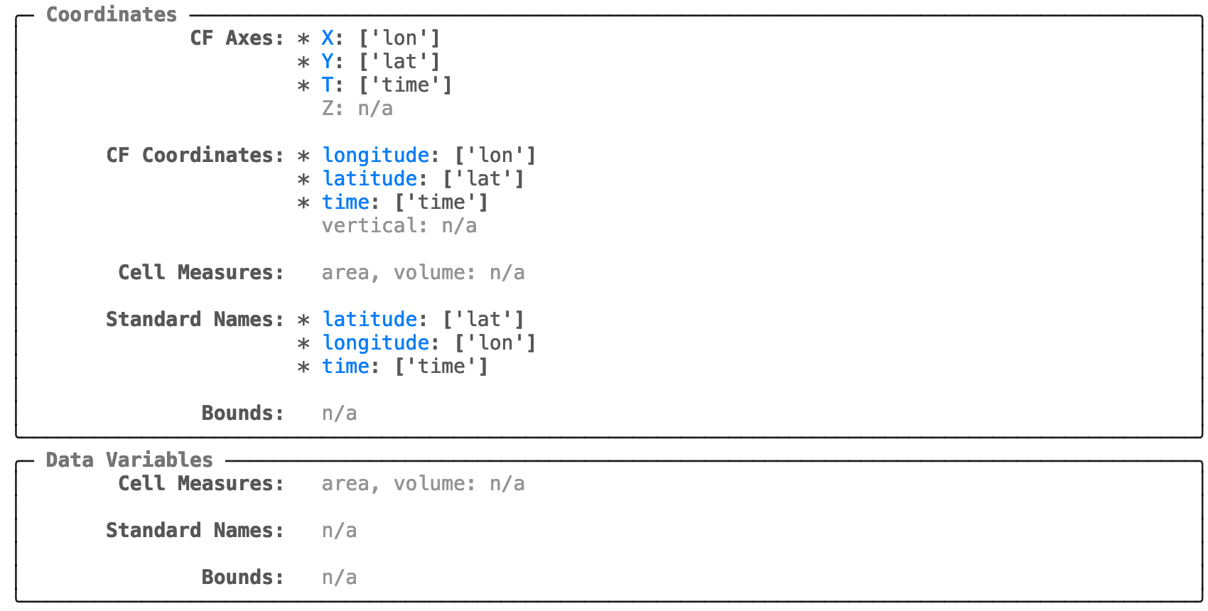
cf_xarray registers an “accessor” named cf on import. For a quick overview of attributes that cf_xarray can interpret use .cf This will display the “repr” or a representation of all detected CF information.
ds.cf
Coordinates:
             CF Axes: * X: ['lon']
                      * Y: ['lat']
                      * T: ['time']
                        Z: n/a

      CF Coordinates: * longitude: ['lon']
                      * latitude: ['lat']
                      * time: ['time']
                        vertical: n/a

       Cell Measures:   area, volume: n/a

      Standard Names: * latitude: ['lat']
                      * longitude: ['lon']
                      * time: ['time']

              Bounds:   n/a

       Grid Mappings:   n/a

Data Variables:
       Cell Measures:   area, volume: n/a

      Standard Names:   n/a

              Bounds:   n/a

       Grid Mappings:   n/a
The plain text repr can be a little hard to read. In a Jupyter environment simply install rich and
use the Jupyter extension with %load_ext rich. Then ds.cf will automatically use the rich representation.
See the rich docs for more.
%load_ext rich

ds.cf
Using attributes
Now instead of the usual xarray names on the right, you can use the “CF names” on the left.
ds.cf.mean("latitude") # identical to ds.mean("lat")
<xarray.Dataset> Size: 1MB
Dimensions:  (time: 2920, lon: 53)
Coordinates:
  * lon      (lon) float32 212B 200.0 202.5 205.0 207.5 ... 325.0 327.5 330.0
  * time     (time) datetime64[ns] 23kB 2013-01-01 ... 2014-12-31T18:00:00
Data variables:
    air      (time, lon) float64 1MB 279.4 279.7 279.7 ... 279.4 280.0 280.5
Attributes:
    Conventions:  COARDS
    title:        4x daily NMC reanalysis (1948)
    description:  Data is from NMC initialized reanalysis\n(4x/day).  These a...
    platform:     Model
references: http://www.esrl.noaa.gov/psd/data/gridded/data.ncep.reanaly...This works because the attributes standard_name: "latitude" and units: "degrees_north" are present on ds.latitude
ds.lat.attrs
{'standard_name': 'latitude',
 'long_name': 'Latitude',
 'units': 'degrees_north',
 'axis': 'Y'}
Tip
For a list of criteria used to identify the “latitude” variable (for e.g.) see Coordinate Criteria.
Similarly we could use ds.cf.mean("Y") because the attribute axis: "Y" is present.
Tip
For best results, we recommend you tell xarray to preserve attributes as much as possible using xr.set_options(keep_attrs=True)
but be warned, this can preserve out-of-date metadata.
Tip
Sometimes datasets don’t have all the necessary attributes. Use guess_coord_axis()
and add_canonical_attributes() to automatically add attributes to variables that match some heuristics.
Indexing
We can use these “CF names” to index into the dataset
ds.cf["latitude"]
<xarray.DataArray 'lat' (lat: 25)> Size: 100B
75.0 72.5 70.0 67.5 65.0 62.5 60.0 57.5 ... 30.0 27.5 25.0 22.5 20.0 17.5 15.0
Coordinates:
  * lat      (lat) float32 100B 75.0 72.5 70.0 67.5 65.0 ... 22.5 20.0 17.5 15.0
Attributes:
    standard_name:  latitude
    long_name:      Latitude
    units:          degrees_north
axis: YThis is particularly useful if a standard_name attribute is present. For demonstration purposes lets add one:
ds.air.attrs["standard_name"] = "air_temperature"
ds.cf["air_temperature"]
<xarray.DataArray 'air' (time: 2920, lat: 25, lon: 53)> Size: 31MB
array([[[241.2 , 242.5 , ..., 235.5 , 238.6 ],
        [243.8 , 244.5 , ..., 235.3 , 239.3 ],
        ...,
        [295.9 , 296.2 , ..., 295.9 , 295.2 ],
        [296.29, 296.79, ..., 296.79, 296.6 ]],

       [[242.1 , 242.7 , ..., 233.6 , 235.8 ],
        [243.6 , 244.1 , ..., 232.5 , 235.7 ],
        ...,
        [296.2 , 296.7 , ..., 295.5 , 295.1 ],
        [296.29, 297.2 , ..., 296.4 , 296.6 ]],

       ...,

       [[245.79, 244.79, ..., 243.99, 244.79],
        [249.89, 249.29, ..., 242.49, 244.29],
        ...,
        [296.29, 297.19, ..., 295.09, 294.39],
        [297.79, 298.39, ..., 295.49, 295.19]],

       [[245.09, 244.29, ..., 241.49, 241.79],
        [249.89, 249.29, ..., 240.29, 241.69],
        ...,
        [296.09, 296.89, ..., 295.69, 295.19],
        [297.69, 298.09, ..., 296.19, 295.69]]], shape=(2920, 25, 53))
Coordinates:
  * lat      (lat) float32 100B 75.0 72.5 70.0 67.5 65.0 ... 22.5 20.0 17.5 15.0
  * lon      (lon) float32 212B 200.0 202.5 205.0 207.5 ... 325.0 327.5 330.0
  * time     (time) datetime64[ns] 23kB 2013-01-01 ... 2014-12-31T18:00:00
Attributes:
    long_name:      4xDaily Air temperature at sigma level 995
    units:          degK
    precision:      2
    GRIB_id:        11
    GRIB_name:      TMP
    var_desc:       Air temperature
    dataset:        NMC Reanalysis
    level_desc:     Surface
    statistic:      Individual Obs
    parent_stat:    Other
    actual_range:   [185.16 322.1 ]
standard_name: air_temperatureFinding variable names
Sometimes it is more useful to extract the actual variable names associated with a given “CF name”. cf_xarray exposes these variable names under a few properties:
These properties all return dictionaries mapping a standard key name to a list of matching variable names in the Dataset or DataArray.
ds.cf.axes
{'X': ['lon'], 'Y': ['lat'], 'T': ['time']}
ds.cf.coordinates
{'longitude': ['lon'], 'latitude': ['lat'], 'time': ['time']}
ds.cf.standard_names
{'air_temperature': ['air'],
 'latitude': ['lat'],
 'longitude': ['lon'],
 'time': ['time']}